
Coordinate-Based Meta-Analysis
Contents
Coordinate-Based Meta-Analysis
# First, import the necessary modules and functions
import os
from pprint import pprint

import matplotlib.pyplot as plt
import numpy as np
from myst_nb import glue
from nilearn import plotting
from repo2data.repo2data import Repo2Data

from nimare import dataset

# Install the data if running locally, or points to cached data if running on neurolibre
DATA_REQ_FILE = os.path.abspath("../binder/data_requirement.json")
repo2data = Repo2Data(DATA_REQ_FILE)
data_path = repo2data.install()
data_path = os.path.join(data_path[0], "data")

# Set an output directory for any files generated during the book building process
out_dir = os.path.abspath("../outputs/")
os.makedirs(out_dir, exist_ok=True)

# Now, load the Datasets we will use in this chapter
sleuth_dset1 = dataset.Dataset.load(os.path.join(data_path, "sleuth_dset1.pkl.gz"))
sleuth_dset2 = dataset.Dataset.load(os.path.join(data_path, "sleuth_dset2.pkl.gz"))
neurosynth_dset = dataset.Dataset.load(os.path.join(data_path, "neurosynth_dataset.pkl.gz"))
---- repo2data starting ----
/srv/conda/envs/notebook/lib/python3.7/site-packages/repo2data
Config from file :
/home/jovyan/binder/data_requirement.json
Destination:
./../data/nimare-paper

Info : ./../data/nimare-paper already downloaded
Coordinate-based meta-analysis (CBMA) is currently the most popular method for neuroimaging meta-analysis, given that the majority of fMRI papers currently report their findings as peaks of statistically significant clusters in standard space and do not release unthresholded statistical maps. These peaks indicate where significant results were found in the brain, and thus do not reflect an effect size estimate for each hypothesis test (i.e., each voxel) as one would expect for a typical meta-analysis. As such, standard methods for effect size-based meta-analysis cannot be applied. Over the past two decades, a number of algorithms have been developed to determine whether peaks converge across experiments in order to identify locations of consistent or specific activation associated with a given hypothesis [Samartsidis et al., 2017, Müller et al., 2018].
Kernel-based methods evaluate convergence of coordinates across studies by first convolving foci with a spatial kernel to produce study-specific modeled activation maps, then combining those modeled activation maps into a sample-wise map, which is compared to a null distribution to evaluate voxel-wise statistical significance. Additionally, for each of the following approaches, except for SCALE, voxel- or cluster-level multiple comparisons correction may be performed using Monte Carlo simulations or false discovery rate (FDR) [Laird et al., 2005] correction. Basic multiple-comparisons correction methods (e.g., Bonferroni correction) are also supported.

Fig. 3 A flowchart of the typical workflow for coordinate-based meta-analyses in NiMARE.
CBMA kernels
CBMA kernels are available as KernelTransformers in the nimare.meta.kernel module.
There are three standard kernels that are currently available: MKDAKernel, KDAKernel, and ALEKernel.
Each class may be configured with certain parameters when a new object is initialized.
For example, MKDAKernel accepts an r parameter, which determines the radius of the spheres that will be created around each peak coordinate.
ALEKernel automatically uses the sample size associated with each experiment in the Dataset to determine the appropriate full-width-at-half-maximum of its Gaussian distribution, as described in Eickhoff et al. [2012]; however, users may provide a constant sample_size or fwhm parameter when sample size information is not available within the Dataset metadata.
Here we show how these three kernels can be applied to the same Dataset.
from nimare.meta import kernel

mkda_kernel = kernel.MKDAKernel(r=10)
mkda_ma_maps = mkda_kernel.transform(sleuth_dset1)
kda_kernel = kernel.KDAKernel(r=10)
kda_ma_maps = kda_kernel.transform(sleuth_dset1)
ale_kernel = kernel.ALEKernel(sample_size=20)
ale_ma_maps = ale_kernel.transform(sleuth_dset1)
# Here we delete the recent variables for the sake of reducing memory usage
del mkda_kernel, kda_kernel, ale_kernel
# Generate figure
study_idx = 10  # a study with overlapping kernels
max_value = np.max(kda_ma_maps[study_idx].get_fdata()) + 1

ma_maps = {
    "MKDA Kernel": mkda_ma_maps[study_idx],
    "KDA Kernel": kda_ma_maps[study_idx],
    "ALE Kernel": ale_ma_maps[study_idx],
}

fig, axes = plt.subplots(nrows=3, figsize=(6, 6))

for i_meta, (name, img) in enumerate(ma_maps.items()):
    if "ALE" in name:
        vmax = None
    else:
        vmax = max_value

    display = plotting.plot_stat_map(
        img,
        annotate=False,
        axes=axes[i_meta],
        cmap="Reds",
        cut_coords=[5, 0, 29],
        draw_cross=False,
        figure=fig,
        vmax=vmax,
    )
    axes[i_meta].set_title(name)

    colorbar = display._cbar
    colorbar_ticks = colorbar.get_ticks()
    if colorbar_ticks[0] < 0:
        new_ticks = [colorbar_ticks[0], 0, colorbar_ticks[-1]]
    else:
        new_ticks = [colorbar_ticks[0], colorbar_ticks[-1]]
    colorbar.set_ticks(new_ticks, update_ticks=True)

glue("figure_ma_maps", fig, display=False)
/srv/conda/envs/notebook/lib/python3.7/site-packages/nilearn/plotting/img_plotting.py:348: FutureWarning: Default resolution of the MNI template will change from 2mm to 1mm in version 0.10.0
  anat_img = load_mni152_template()

# Here we delete the recent variables for the sake of reducing memory usage
del mkda_ma_maps, kda_ma_maps, ale_ma_maps
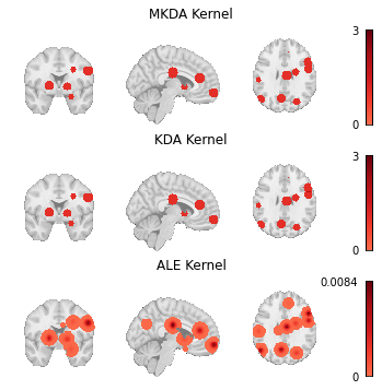
Fig. 4 Modeled activation maps produced by NiMARE’s KernelTransformer classes.
from nimare import dataset, meta

neurosynth_dset_first500 = dataset.Dataset.load(
    os.path.join(data_path, "neurosynth_dataset_first500.pkl.gz")
)

# Specify where images for this Dataset should be located
target_folder = os.path.join(out_dir, "neurosynth_dataset_maps")
os.makedirs(target_folder, exist_ok=True)
neurosynth_dset_first500.update_path(target_folder)

# Initialize a kernel transformer to use
kern = meta.kernel.MKDAKernel(memory_limit="500mb")

# Run the kernel transformer with return_type set to "dataset" to return an updated Dataset
# with the MA maps stored as files within its "images" attribute.
neurosynth_dset_first500 = kern.transform(neurosynth_dset_first500, return_type="dataset")
neurosynth_dset_first500.save(
    os.path.join(out_dir, "neurosynth_dataset_first500_with_mkda_ma.pkl.gz"),
)
INFO:nimare.utils:Shared path detected: '/home/jovyan/outputs/neurosynth_dataset_maps/'
Multilevel kernel density analysis
Multilevel kernel density analysis (MKDA) [Wager et al., 2007] is a kernel-based method that convolves each peak from each study with a binary sphere of a set radius. These peak-specific binary maps are then combined into study-specific maps by taking the maximum value for each voxel. Study-specific maps are then averaged across the meta-analytic sample. This averaging is generally weighted by studies’ sample sizes, although other covariates may be included, such as weights based on the type of inference (random or fixed effects) employed in the study’s analysis. An arbitrary threshold is generally employed to zero-out voxels with very low values, and then a Monte Carlo procedure is used to assess statistical significance, either at the voxel or cluster level.
In NiMARE, the MKDA meta-analyses can be performed with the MKDADensity class.
This class, like most other CBMA classes in NiMARE, accepts a null_method parameter, which determines how voxel-wise (uncorrected) statistical significance is calculated.
On CBMA “null methods”
The null_method parameter allows two options: “approximate” or “montecarlo.”
The “approximate” option builds a histogram-based null distribution of summary-statistic values, which can then be used to determine the associated p-value for observed summary-statistic values (i.e., the values in the meta-analytic map).
The “montecarlo” option builds a null distribution of summary-statistic values by randomly shuffling the coordinates the Dataset many times, and computing the summary-statistic values for each permutation.
In general, the “montecarlo” method is slightly more accurate when there are enough permutations, while the “approximate” method is much faster.
Warning
Fitting the CBMA Estimator to a Dataset will produce p-value, z-statistic, and summary-statistic maps, but these are not corrected for multiple comparisons.
When performing a meta-analysis with the goal of statistical inference, you will want to perform multiple comparisons correction with NiMARE’s Corrector
classes.
Please see the multiple comparisons correction chapter for more information.
Here we perform an MKDADensity meta-analysis on one of the Sleuth-based Datasets. We will use the “approximate” null method for speed.
from nimare.meta.cbma import mkda

mkdad_meta = mkda.MKDADensity(null_method="approximate")
mkdad_results = mkdad_meta.fit(sleuth_dset1)
The MetaResult class
Fitting an Estimator to a Dataset produces a MetaResult object.
The MetaResult class is a light container holding the different statistical maps produced by the Estimator.
print(mkdad_results)
<nimare.results.MetaResult object at 0x7fe832142390>
This result is also retained as an attribute in the Estimator.
print(mkdad_meta.results)
<nimare.results.MetaResult object at 0x7fe832142390>
The maps attribute is a dictionary containing statistical map names and associated numpy arrays.
pprint(mkdad_results.maps)
{'p': array([1., 1., 1., ..., 1., 1., 1.]),
 'stat': array([0., 0., 0., ..., 0., 0., 0.]),
 'z': array([0., 0., 0., ..., 0., 0., 0.])}
These arrays can be transformed into image-like objects using the masker attribute.
We can also use the get_map method to get that image object.
mkdad_img = mkdad_results.get_map("z", return_type="image")
print(mkdad_img)
<class 'nibabel.nifti1.Nifti1Image'>
data shape (91, 109, 91)
affine:
[[  -2.    0.    0.   90.]
 [   0.    2.    0. -126.]
 [   0.    0.    2.  -72.]
 [   0.    0.    0.    1.]]
metadata:
<class 'nibabel.nifti1.Nifti1Header'> object, endian='<'
sizeof_hdr      : 348
data_type       : b''
db_name         : b''
extents         : 0
session_error   : 0
regular         : b''
dim_info        : 0
dim             : [  3  91 109  91   1   1   1   1]
intent_p1       : 0.0
intent_p2       : 0.0
intent_p3       : 0.0
intent_code     : none
datatype        : float64
bitpix          : 64
slice_start     : 0
pixdim          : [-1.  2.  2.  2.  1.  1.  1.  1.]
vox_offset      : 0.0
scl_slope       : nan
scl_inter       : nan
slice_end       : 0
slice_code      : unknown
xyzt_units      : 0
cal_max         : 0.0
cal_min         : 0.0
slice_duration  : 0.0
toffset         : 0.0
glmax           : 0
glmin           : 0
descrip         : b''
aux_file        : b''
qform_code      : unknown
sform_code      : aligned
quatern_b       : 0.0
quatern_c       : 1.0
quatern_d       : 0.0
qoffset_x       : 90.0
qoffset_y       : -126.0
qoffset_z       : -72.0
srow_x          : [-2.  0.  0. 90.]
srow_y          : [   0.    2.    0. -126.]
srow_z          : [  0.   0.   2. -72.]
intent_name     : b''
magic           : b'n+1'
We can save the statistical maps to an output directory as gzipped nifti files, with a prefix. Here, we will save all of the statistical maps with the MKDADensity prefix.
mkdad_results.save_maps(output_dir=out_dir, prefix="MKDADensity")
We will also save the Estimator itself, which we will reuse when we get to multiple comparisons correction.
mkdad_meta.save(os.path.join(out_dir, "MKDADensity.pkl.gz"))
# Here we delete the recent variables for the sake of reducing memory usage
del mkdad_meta, mkdad_results
Since this is a kernel-based algorithm, the kernel transformer is an optional input to the meta-analytic estimator, and can be controlled in a more fine-grained manner.
# These two approaches (initializing the kernel ahead of time or
# providing the arguments with the kernel__ prefix) are equivalent.
mkda_kernel = kernel.MKDAKernel(r=2)
mkdad_meta = mkda.MKDADensity(kernel_transformer=mkda_kernel)
mkdad_meta = mkda.MKDADensity(kernel_transformer=kernel.MKDAKernel, kernel__r=2)

# A completely different kernel could even be provided, although this is not
# recommended and should only be used for testing algorithms.
mkdad_meta = mkda.MKDADensity(kernel_transformer=kernel.KDAKernel)
WARNING:nimare.meta.cbma.mkda:The KernelTransformer being used (<class 'nimare.meta.kernel.KDAKernel'>) is not optimized for the MKDADensity algorithm. Expect suboptimal performance and beware bugs.
# Here we delete the recent variables for the sake of reducing memory usage
del mkda_kernel, mkdad_meta
Kernel density analysis
Kernel density analysis (KDA) [Wager et al., 2003, Wager et al., 2004] is a precursor algorithm that has been replaced in the field by MKDA. For the sake of completeness, NiMARE also includes a KDA estimator that implements the older KDA algorithm for comparison purposes. The interface is virtually identical, but since there are few if any legitimate uses of KDA (which models studies as fixed rather than random effects), we do not discuss the algorithm further here.
kda_meta = mkda.KDA(null_method="approximate")
kda_results = kda_meta.fit(sleuth_dset1)

# Retain the z-statistic map for later use
kda_img = kda_results.get_map("z", return_type="image")
WARNING:nimare.meta.cbma.mkda:The KDA algorithm has been replaced in the literature with the MKDA algorithm. As such, this estimator should almost never be used, outside of systematic comparisons between algorithms.
# Here we delete the recent variables for the sake of reducing memory usage
del kda_meta, kda_results
Activation likelihood estimation
Activation likelihood estimation (ALE) [Eickhoff et al., 2012, Turkeltaub et al., 2012, Turkeltaub et al., 2002] assesses convergence of peaks across studies by first generating a modeled activation map for each study, in which each of the experiment’s peaks is convolved with a 3D Gaussian distribution determined by the experiment’s sample size, and then by combining these modeled activation maps across studies into an ALE map, which is compared to an empirical null distribution to assess voxel-wise statistical significance.
from nimare.meta.cbma import ale

ale_meta = ale.ALE()
ale_results = ale_meta.fit(sleuth_dset1)

# Retain the z-statistic map for later use
ale_img = ale_results.get_map("z", return_type="image")
# Here we delete the recent variables for the sake of reducing memory usage
del ale_meta, ale_results
Specific coactivation likelihood estimation
Specific coactivation likelihood estimation (SCALE) [Langner et al., 2014] is an extension of the ALE algorithm developed for meta-analytic coactivation modeling (MACM) analyses. Rather than comparing convergence of foci within the sample to a null distribution derived under the assumption of spatial randomness within the brain, SCALE assesses whether the convergence at each voxel is greater than in the general literature. Each voxel in the brain is assigned a null distribution determined based on the base rate of activation for that voxel across an existing coordinate-based meta-analytic database. This approach allows for the generation of a statistical map for the sample, but no methods for multiple comparisons correction have yet been developed. While this method was developed to support analysis of joint activation or “coactivation” patterns, it is generic and can be applied to any CBMA; see Derivative Analyses
# Here we use the coordinates from Neurosynth as our measure of coordinate
# base-rates, because we do not have access to the full BrainMap database.
# However, one assumption of SCALE is that the Dataset being analyzed comes
# from the same source as the database you use for calculating base-rates.
xyz = neurosynth_dset.coordinates[["x", "y", "z"]].values
# Typically, you would have >=2500 iterations, but we're using 500 here.
scale_meta = ale.SCALE(n_iters=500, xyz=xyz, memory_limit="100mb", n_cores=1)
scale_results = scale_meta.fit(sleuth_dset1)

# Retain the z-statistic map for later use
scale_img = scale_results.get_map("z", return_type="image")
# Here we delete the recent variables for the sake of reducing memory usage
del xyz, scale_meta, scale_results
MKDA Chi-Squared Analysis
An alternative to the density-based approaches (i.e., MKDA, KDA, ALE, and SCALE) is the MKDA Chi-squared extension [Wager et al., 2007]. Though still a kernel-based method in which foci are convolved with a binary sphere and combined within studies, this approach uses voxel-wise chi-squared tests to assess both consistency (i.e., higher convergence of foci within the meta-analytic sample than expected by chance) and specificity (i.e., higher convergence of foci within the meta-analytic sample than detected in an unrelated dataset) of activation. Such an analysis also requires access to a reference meta-analytic sample or database of studies. For example, to perform a chi-squared analysis of working memory studies, the researcher will also need a comprehensive set of studies which did not manipulate working memory—ideally one that is matched with the working memory study set on all relevant attributes except the involvement of working memory.
mkdac_meta = mkda.MKDAChi2()
mkdac_results = mkdac_meta.fit(sleuth_dset1, sleuth_dset2)

# Retain the specificity analysis's z-statistic map for later use
mkdac_img = mkdac_results.get_map("z_desc-specificity", return_type="image")
/srv/conda/envs/notebook/lib/python3.7/site-packages/nimare/meta/cbma/mkda.py:276: RuntimeWarning: invalid value encountered in true_divide
  pFgA = pAgF * pF / pA
/srv/conda/envs/notebook/lib/python3.7/site-packages/nimare/meta/cbma/mkda.py:280: RuntimeWarning: invalid value encountered in true_divide
  pFgA_prior = pAgF * self.prior / pAgF_prior
# Here we delete the recent variables for the sake of reducing memory usage
del mkdac_meta, mkdac_results
Comparing algorithms
Here we load the z-statistic map from each of the CBMA Estimators we’ve used throughout this chapter and plot them all side by side.
meta_results = {
    "MKDA Density": mkdad_img,
    "MKDA Chi-Squared": mkdac_img,
    "KDA": kda_img,
    "ALE": ale_img,
    "SCALE": scale_img,
}
order = [
    ["MKDA Density", "ALE"],
    ["MKDA Chi-Squared", "SCALE"],
    ["KDA", None]
]

fig, axes = plt.subplots(figsize=(12, 6), nrows=3, ncols=2)

for i_row, row_names in enumerate(order):
    for j_col, name in enumerate(row_names):
        if not name:
            axes[i_row, j_col].axis("off")
            continue

        img = meta_results[name]
        if name == "MKDA Chi-Squared":
            cmap = "RdBu_r"
        else:
            cmap = "Reds"

        display = plotting.plot_stat_map(
            img,
            annotate=False,
            axes=axes[i_row, j_col],
            cmap=cmap,
            cut_coords=[5, -15, 10],
            draw_cross=False,
            figure=fig,
        )
        axes[i_row, j_col].set_title(name)

        colorbar = display._cbar
        colorbar_ticks = colorbar.get_ticks()
        if colorbar_ticks[0] < 0:
            new_ticks = [colorbar_ticks[0], 0, colorbar_ticks[-1]]
        else:
            new_ticks = [colorbar_ticks[0], colorbar_ticks[-1]]
        colorbar.set_ticks(new_ticks, update_ticks=True)

glue("figure_cbma_uncorr", fig, display=False)
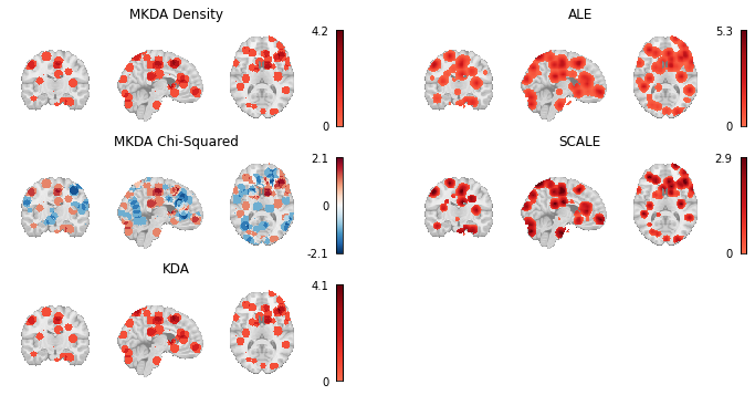

Fig. 5 Thresholded results from MKDA Density, KDA, ALE, and SCALE meta-analyses.
A number of other coordinate-based meta-analysis algorithms exist which are not yet implemented in NiMARE. We describe these algorithms briefly in Future Directions.